Different types of oscillators for digital audio synthesis.
Oscillators are the heart of any synthesizer as they are used both to generate sound waves and to modulate parameters related to those sound waves to produce more complex timbres and evolving sounds. In what follows we will be plotting various kinds of wave shapes we want to use for our oscillators. If we can generate a single cycle of our wave over the range [0,1], then we can easily extend it to any pitch by sampling either faster or slower from that shape. We will use some of our linear-algebra tools to derive these.
Implementing Oscillators
In order to derive the wave shapes for our oscillators we will need to lay down some constraints. First, each oscillator function must return results in the range [-1.0, 1.0]. These values can then have local and global amplitude (volume) adjustments applied before generating samples (like 16-bit stereo samples).
Second, some assumptions about the implementation. To produce audio we must generate sampled sound waves in PCM format. The sampling rate (in Hertz or Hz) tells us how many samples compose a single second of audio. This allows us to determine (for a given pitch or frequency) how quickly we must loop through the waveform to produce sound at that pitch. Therefore, one important piece of global state is the sampling rate. It can be defined along with some useful constants something like the following:
/* Header file somewhere */
#define G_PI 3.14159265358
#define G_TAU 6.28318530718

extern double gSamplingRate;

/* Source file somewhere */
double gSamplingRate = 48000.0; /* Could also be 44100.0 */
The basic structure of an oscillator below will involve the following per-oscillator state:
typedef enum Wave_Shape Wave_Shape;
enum Wave_Shape {
  	WAVESHAPE_sine,
  	WAVESHAPE_square,
  	WAVESHAPE_sawtooth,
  	WAVESHAPE_triangle,

	WAVESHAPE_COUNT
};

typedef struct Oscillator Oscillator;
struct Oscillator {
	Wave_Shape	WaveShape;
	double		FrequencyHz;
	double		DutyCycle; /* Square wave only (value in range [0.0, 100.0]) */

	double		Value;
	double		Phase;
	double		PhaseIncrement;
	double		Period;
	double		MidPoint;
}
Where Value is the current value in the range [-1.0, 1.0], Phase is a value indicating progress through a single cycle, and PhaseIncrement is the value used to advance the phase by a single sample. Period is the value of Phase when it has reached the end of the cycle and is used to reset Phase to start another loop through the waveform. Some oscillators may have additional state data (ex. square waves have a DutyCycle and use MidPoint).
Finally, each wave shape will implement the following two methods. Where Reset initializes the oscillator state for the given wave shape and frequency and Tick advances the oscillator by one sample. Typically all the oscillators will just be implemented in a giant switch on WaveShape:
void OscillatorReset(Oscillator* osc);
void OscillatorTick(Oscillator* osc);
Sine Wave
/* Oscillator implementations for Sine Wave */

void OscillatorReset(Oscillator* osc) {
	/* Clamp the frequency of the oscillator to the Nyquist frequency */
	double half_sample_rate = gSamplingRate / 2.0;
	double clamped_freq = fmin(osc->FrequencyHz, half_sample_rate);

	osc->Value = 0.0;
	osc->Phase = 0.0;

	osc->PhaseIncrement = (clamped_freq * G_TAU) / gSamplingRate;
	osc->Period = G_TAU;
}

void OscillatorTick(Oscillator* osc) {
	osc->Value = sin(osc->Phase);

	osc->Phase += osc->PhaseIncrement;
	if (osc->Phase >= osc->Period) {
		osc->Phase -= osc->Period;
	}
}
The unit sine wave is shown below:
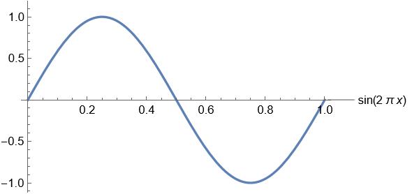
What we notice is that for each unit x that we want to advance we actually want to increase the input by 2 * PI * x. This informs our selection of value for the PhaseIncrement (G_TAU is just 2 * PI).
Square Wave
/* Oscillator implementations for Square Wave */

void OscillatorReset(Oscillator* osc) {
	/* Clamp the frequency of the oscillator to the Nyquist frequency */
	double half_sample_rate = gSamplingRate / 2.0;
	double clamped_freq = fmin(osc->FrequencyHz, half_sample_rate);

	osc->Value = 0.0;
	osc->Phase = 0.0;

	osc->PhaseIncrement = 1.0 / gSamplingRate;
	osc->Period = 1.0 / clamped_freq;
	osc->MidPoint = osc->Period * osc->DutyCycle / 100.0;
}

void OscillatorTick(Oscillator* osc) {
	osc->Value = (osc->Phase < osc->MidPoint) ? 1.0 : -1.0;

	osc->Phase += osc->PhaseIncrement;
	if (osc->Phase >= osc->Period) {
		osc->Phase -= osc->Period;
	}
}
The simplest square wave is one that assumes its highest value during half a cycle and its lowest value the other half as follows:
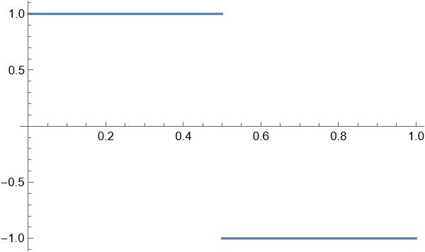
However, we can also modulate the width of this square wave to produce timbral variety in our sounds. The percent of the time spent at the highest value is called the duty cycle (Dc) and is restricted to the range [0,1] where zero is always low and one is always high. We can see a few different duty cycles below:
| Dc = 12.5% | 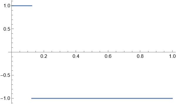 |
| Dc = 50.0% | |
| Dc = 87.5% | 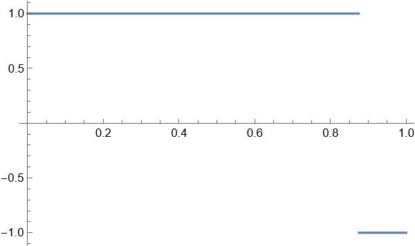 |
Sawtooth Wave
The implementation of the interface for a sawtooth wave can be seen below:
/* Oscillator implementations for Sawtooth Wave */

void OscillatorReset(Oscillator* osc) {
	/* Clamp the frequency of the oscillator to the Nyquist frequency */
	double half_sample_rate = gSamplingRate / 2.0;
	double clamped_freq = fmin(osc->FrequencyHz, half_sample_rate);

	osc->Value = 0.0;
	osc->Phase = 0.0;

	osc->PhaseIncrement = 2.0 * clamped_freq / gSamplingRate;
	osc->Period = 2.0;
}

void OscillatorTick(Oscillator* osc) {
	osc->Value = osc->Phase - 1.0;

	osc->Phase += osc->PhaseIncrement;
	if (osc->Phase >= osc->Period) {
		osc->Phase -= osc->Period;
	}
}
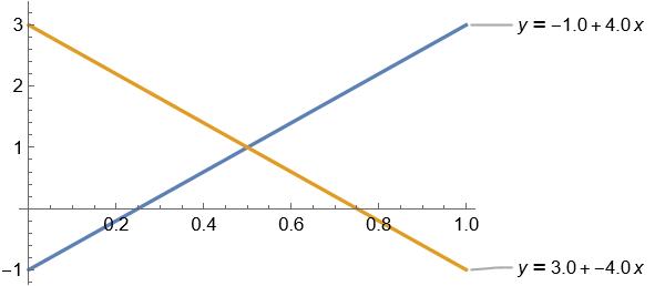
To derive this we will start from a typical sawtooth wave shown below:
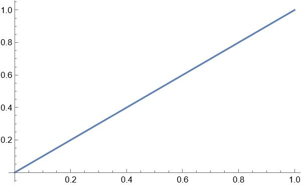
This is a simple line, however we would like to change the range from [0,1] to [-1,1]. We can derive the formula for it by solving the following system of linear equations:
0m + b = -1
1m + b = 1
We can rewrite this as a homogeneous system and row reduce (using our Gaussian Elimination system):
double matrix[3][3] = {
  {0.0, 1.0, 1.0},
  {1.0, 1.0, -1.0}
}
This produces the following solution:
[0.00	1.00	1.00]
[1.00	1.00	-1.00]

[1.00	0.00	-2.00]
[0.00	1.00	1.00]
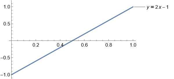
Giving us the linear equation y = 2x - 1, which looks like this:
Triangle Wave
The implementation of the interface for a triangle wave can be seen below:
/* Oscillator implementations for Triangle Wave */

void OscillatorReset(Oscillator* osc) {
	/* Clamp the frequency of the oscillator to the Nyquist frequency */
	double half_sample_rate = gSamplingRate / 2.0;
	double clamped_freq = fmin(osc->FrequencyHz, half_sample_rate);

	osc->Value = 0.0;
	osc->Phase = 0.0;

	osc->PhaseIncrement = 4.0 * clamped_freq / gSamplingRate;
	osc->Period = 4.0;
}

void OscillatorTick(Oscillator* osc) {
	if (osc->Phase < 2.0) {
		osc->Value = osc->Phase - 1.0;
	} else {
		osc->Value = 3.0 - osc->Phase;
	}

	osc->Phase += osc->PhaseIncrement;
	if (osc->Phase >= osc->Period) {
		osc->Phase -= osc->Period;
	}
}
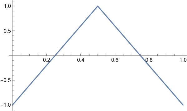
A typical graph of a triangle wave looks something like this:
However to approximate on the range [0,1] we would need a piecewise function of three linear equations (these can be derived using the same linear algebra methods above) as follows:
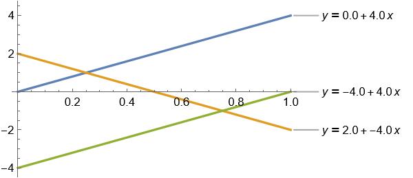
Zooming in a bit we can see our original triangle wave:
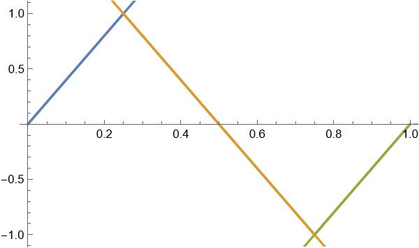
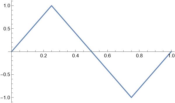
We can simplify this if we shift the original triangle wave to the right 0.25 units as follows:
We can see that this exactly maps to a piecewise function of only two linear equations: